Extended usage

Create a new Pecube project

To create and run a new Pecube project, go to New input file or press Crtl+N (3, see Introduction), a window pops up and asks you to provide the name of the new project (Figure 1). Pecube requires that the project name be 5 characters length. After clicking the “Ok” button (Figure 2), you will be able to provide and set all of the Pecube input parameters for your project.

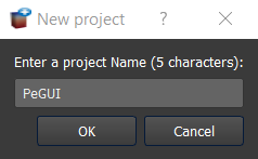
Figure 1. Enter a new project name. This window shows up when clicking on the “New input file” action button.

The window should look like Figure 2. On the top left, you could find and access all the projects you have loaded into the interface, and thus navigate through their respective parameters. The right part of the interface will host extra input parameters described in the next sections.

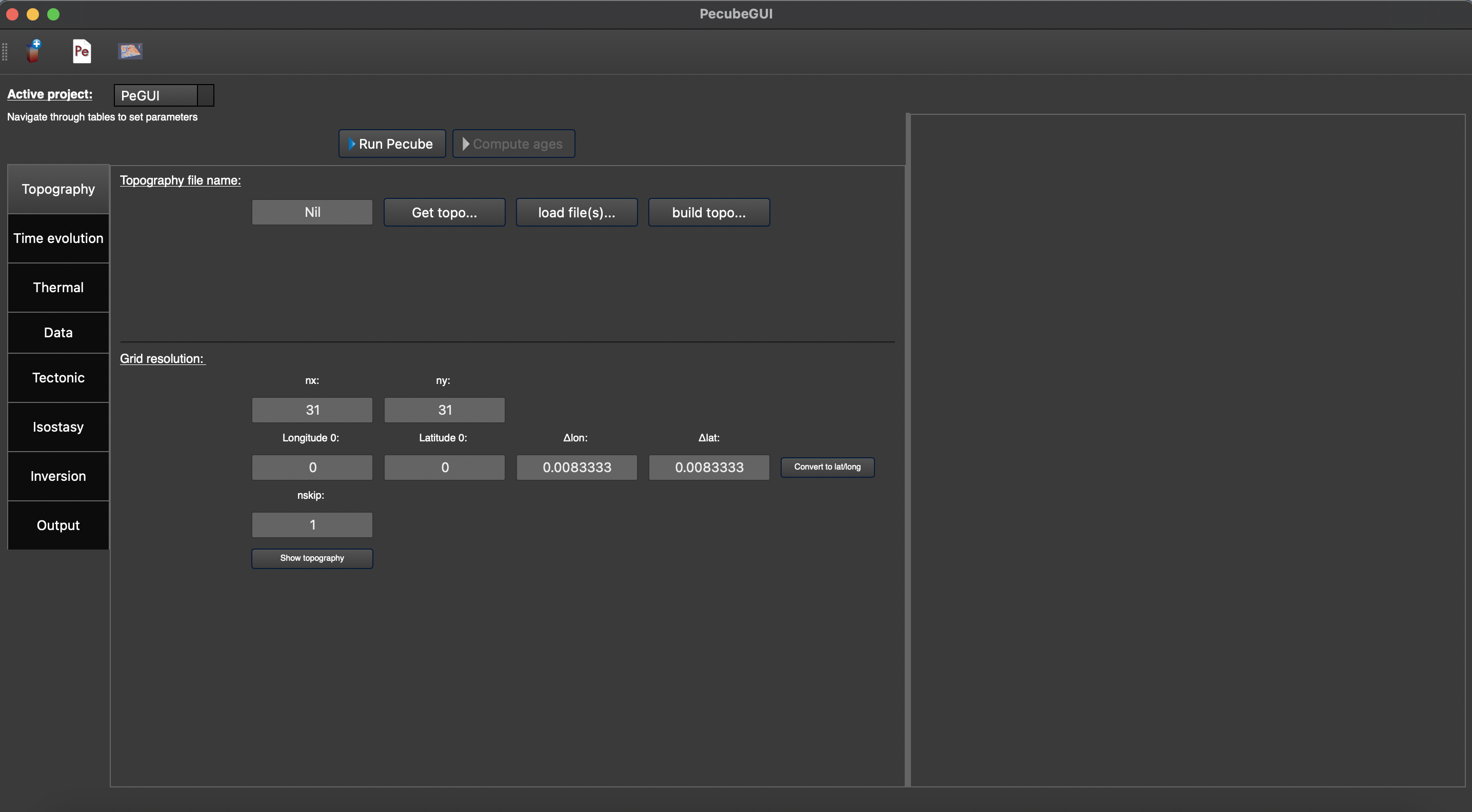
Figure 2. Tab to set up the input parameters for Pecube. On the top left, you can check the name of your project (here: ‘PeGUI’)

The input parameters are organised into categories similar to what is referenced in the Pecube’s user guide (in ‘Pecube/docs/Pecube.pdf’). All the parameters are sorted in 8 categories: Topography, Time evolution, Thermal, Data, Tectonic, Isostasy, Inversion, and Output parameters. For more details on the meaning of each input parameter please refer to the Pecube’s user guide. However, you could access to a short description of each parameter by simply flying the mouse cursor over the parameter labels. After one second a text should appear and describe the parameter.

In the following, I provide a description of all the tabs, and how to provide the input parameters in PecubeGUI.

Provide input parameters

Topography tab

---

When providing the project name, you will automatically be directed to the first tab that shows the “Topography” parameters (Figure 2). All the default values of the input parameters are displayed, so that you do not need to provide them if you want to keep these default values. If you wish to change a parameter, simply click on the text box, and write your value.

PecubeGUI offers the possibility to simply load topographic file(s) from:

• a txt file containing one column of elevation

• a serie of output files from a spm to be read by Pecube (see Pecube user guide – “Topography parameters”)

• a DEM file (i.e., raster file ‘.tif’)

• a DEM extracted OpenTopography (“Get topo…”, Fig. 2)

• You can also choose to build a simple sinusoïdal topography (‘Build topo…”, Fig. 2).

For the three first points, clicking on ‘load file(s)’ (Figure 2) will allow you to select the file(s) to load. A window pops up. The figure 3 shows an example where a serie of files has been loaded from a spm like iSOSIA [Egholm_et-al-2011].

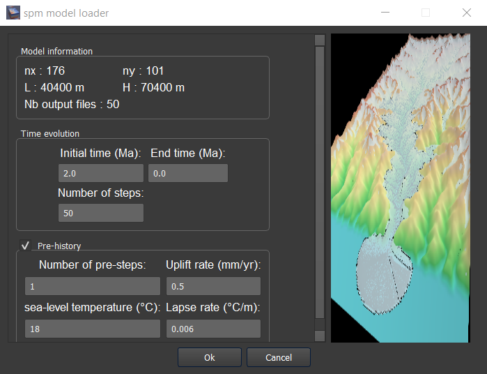
Figure 3. Spm loader window.

This window recovers some characteristics of your spm model, which are shown on the top for checking (works for iSOSIA models only). Then, you are asked to provide the starting and ending times of your model (in Ma), as well as the number of steps (i.e., the number of topographic files). The initial time is older than the end time. This is required to automatically set the time values for the “Time evolution” tab.

You are also able to provide a simple pre-spm history for the topographic evolution. For that purpose, click on “Pre-history” (Figure 3). You will be able to provide 4 parameters:

• number of pre-steps: how many steps for the pre-spm history you want to provide topographic information

• uplift rate: this will be assumed to be spatially uniform and applied to all pre-history steps

• sea-level temperature

• atmospheric lapse rate

PecubeGUI will start from the first topographic file provided and interpolate back the pre-spm topographic history according to the amplitude and offset parameters you will provide in the next steps (see Time evolution tab).

After clicking the “Ok” button, the files will be copied and pasted into “your_current_project_path\data\SPM”. In the meantime, the name “SPM/” is automatically provided to the input parameters “Topography file name”, as well as the grid resolution (i.e., nx and ny, works only with iSOSIA files, Figure 3).

When loading a synthetic numerical model, you can let the latitude and longitude to zero. However, you need to provide the stepping distance in x (Δlon) and y (Δlat). For simplicity, you can provide the values in km and then click on ‘Convert to lat/long’ button (Figure 2). This will automatically convert the values to longitude and latitude distances that can be read by Pecube.

Alternatively, you can extract a DEM from OpenTopography. To do so, you will need first to request an API key from OpenTopography website (request api key ). Then copy your key in a text file, name it “OpenTopoKey.txt”, and put the file in the root directory of PecubeGUI application (i.e., the same location than the Pecube directory). To download a DEM of your region of interest (ROI), provide the coordinates of the bottom left corner of the topography and its resolution in the “Topography” tab (i.e., nx, ny, longitude 0, latitude 0, Δlon, Δlat). Click on “Get topo…” button will then extract the DEM. This option uses the python package bmi_topography [Piper-2021] to download the DEM from the SRTMGL3 (90 m resolution) hosted by OpenTopography. According to the size of your ROI it can take few second to download. Once the DEM is downloaded, it can be found in “your_current_project/data/” directory. Click on “load file(s)” (Figure 2) to load the DEM within the interface.

Important

If you use the DEM from the SRTM data hosted by OpenTopography, please use this citation: NASA Shuttle Radar Topography Mission (SRTM) (2013). Shuttle Radar Topography Mission (SRTM) Global. Distributed by OpenTopography. https://doi.org/10.5069/G9445JDF. Accessed: 2022-11-18. With the in-text citation: NASA Shuttle Radar Topography Mission (2013).

You can also decide to build a simple sinusoïdal topography. For this purpose, click on “Build topo…” (Figure 2). A window pops up in which you can set the dimension and resolution of the synthetic topography as well as the amplitude, wavelength, and a phase shift (Figure 5). When you are done, click on “Ok” and the topography will be automatically loaded within the interface.

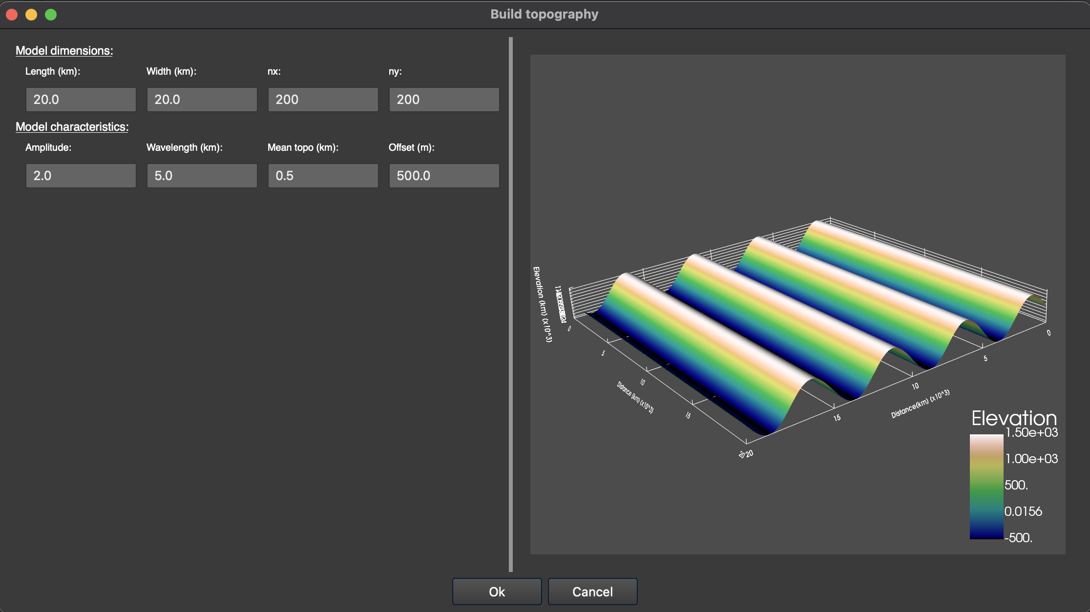
Figure 5. Window showing up when clicking on ‘build topo…” (Figure 2) to build a synthetic sinusoïdal topography.

Finally, you can check your input topography by clicking on “Show topography” (Figure 2). A new tab appears on the right-hand side of the interface (Figure 6). This tab serves to visualize the topography and check your topography history as provided in the Time evolution tab. For this, simply grab and drag the slide bar in “Set time evolution” (Figure 6).

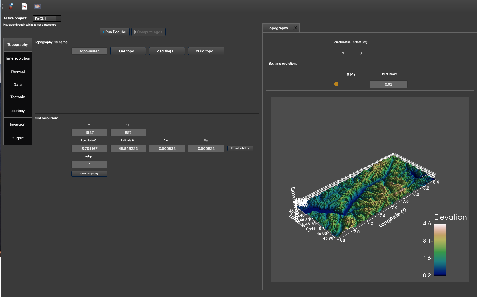
Figure 6. “Topography” tab with the topography shown on the right-hand side, after clicking the “Show topogaphy” button. Here, the topography is loaded from a DEM from the Rhone valley in Switzerland.

Time evolution tab

---

In this tab (Figure 7) you can provide all the parameters controlling the time evolution of the input topography. In PecubeGUI you can provide the time evolution parameters (cf. “time_topo”,” amplification”, “offset”, and “output”) by filling in the table or by copying/pasting values from an excel file to the table. The number of rows in the table automatically updates from the value written in the parameter “ntime” (Figure 7).

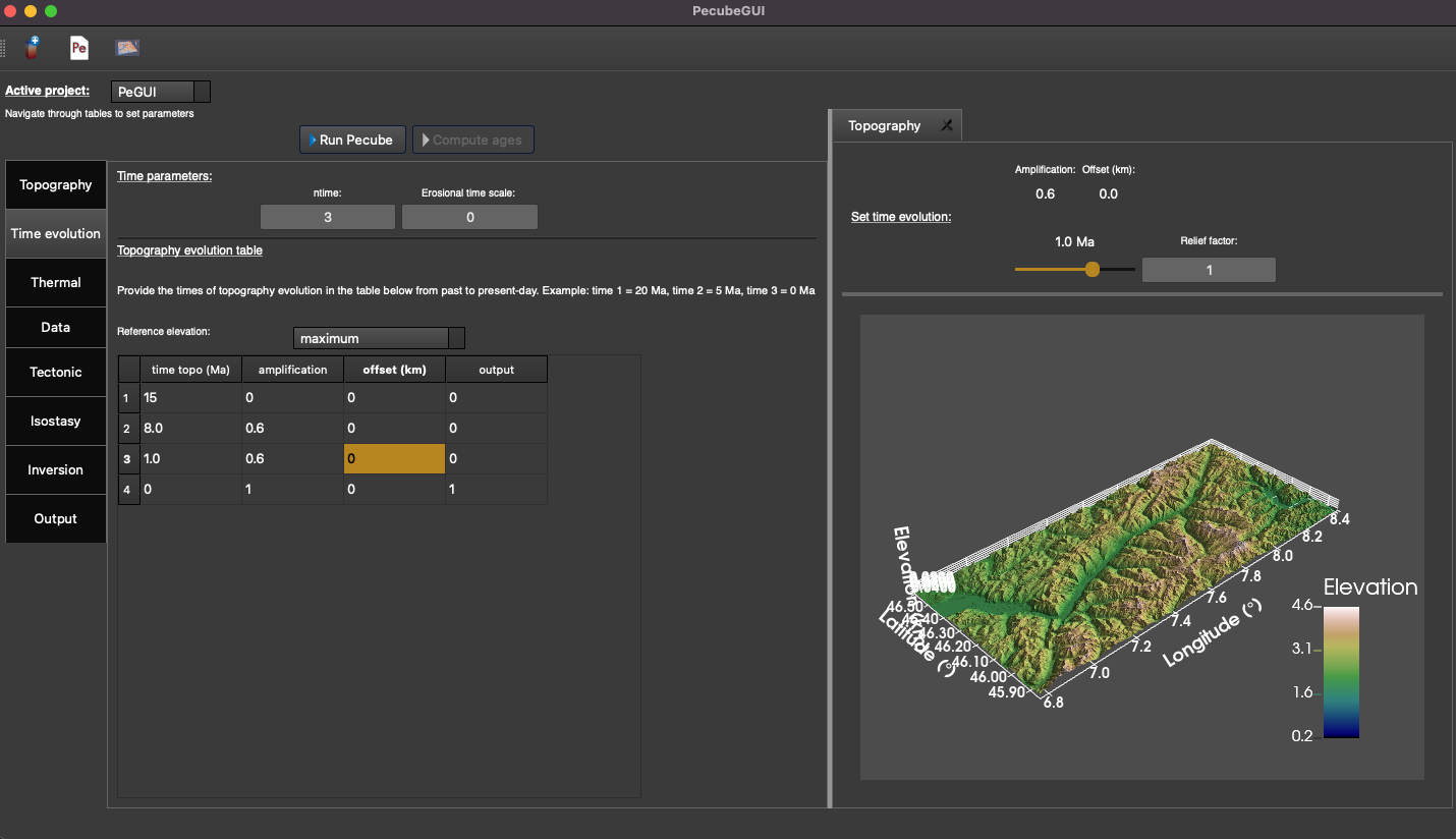
Figure 7. “Time evolution” tab where to provide the parameters related to the time evolution of the topography. In this example, the topography evolution is defined relative to the maximum elevation.

The default value for each parameter is also automatically provided.

In the previous versions of Pecube, one could provide a topography as input and set its evolution through time by varying the amplification and offset parameters, according to the following equation:

h_i= offset_i + amplification_i * h₀

The formulation of the above equation has been modified in PecubeGUI to allow for choosing the reference elevation from which to apply the relief amplification factor. One can now choose to have the sea level, minimum, maximum, or mean elevation as a reference (see Figure 8). The topographic evolution now follows:

h_i= offset_i + topo_ref - [amplification_i * (topo_ref - h₀)]

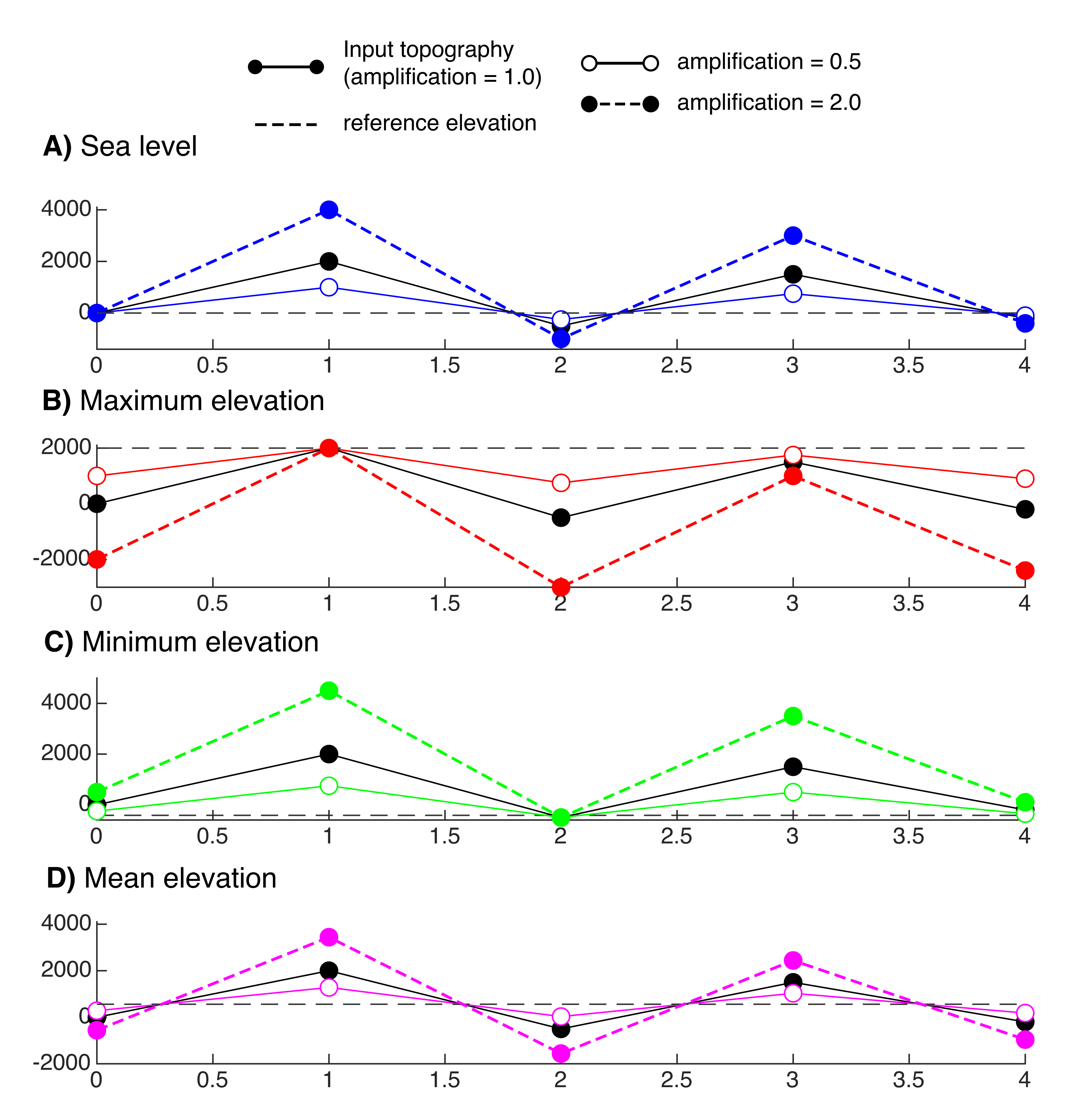
Figure 8. Reference elevations from which to apply the relief amplification factor. These references are A) sea level, B) minimum, C) maximum, D) mean elevation.

Thermal tab

---

The Thermal tab gathers all the parameters to set the thermal properties of the crust and the atmosphere of a Pecube model. In PecubeGUI, the user can check for the 1D steady-state geotherm by simply clicking on “Show Geotherm” (Figure 9). A new tab appears on the right-hand side of the interface, where the geotherm is shown. In addition, the user can check the influence of the erosion rate on the geotherm by providing values in “Mean erosion rate” (Figure 9, only for visual purposes). The 1D steady-state geotherm is computed using the equation found in [Reiners-and-Brandon-2006] that accounts for the effect of erosion rates on the thermal state of the crust.

Moreover, the user can provide the specific heat capacity (J.kg^-1.K^-1) and the radioactive heat production (µW.m^-3). The equivalent heat production rate (°C.Myr^-1) will automatically be updated (Figure 9). Finally, the resulting surface heat flux is shown as a checking.

The user can also set a non-uniform heat production rate. An exponential decrease of heat production rate with depth can be specified by checking the box “use e-folding HP”. A small window pops up where you can provide the heat production rate and the e-folding depth.

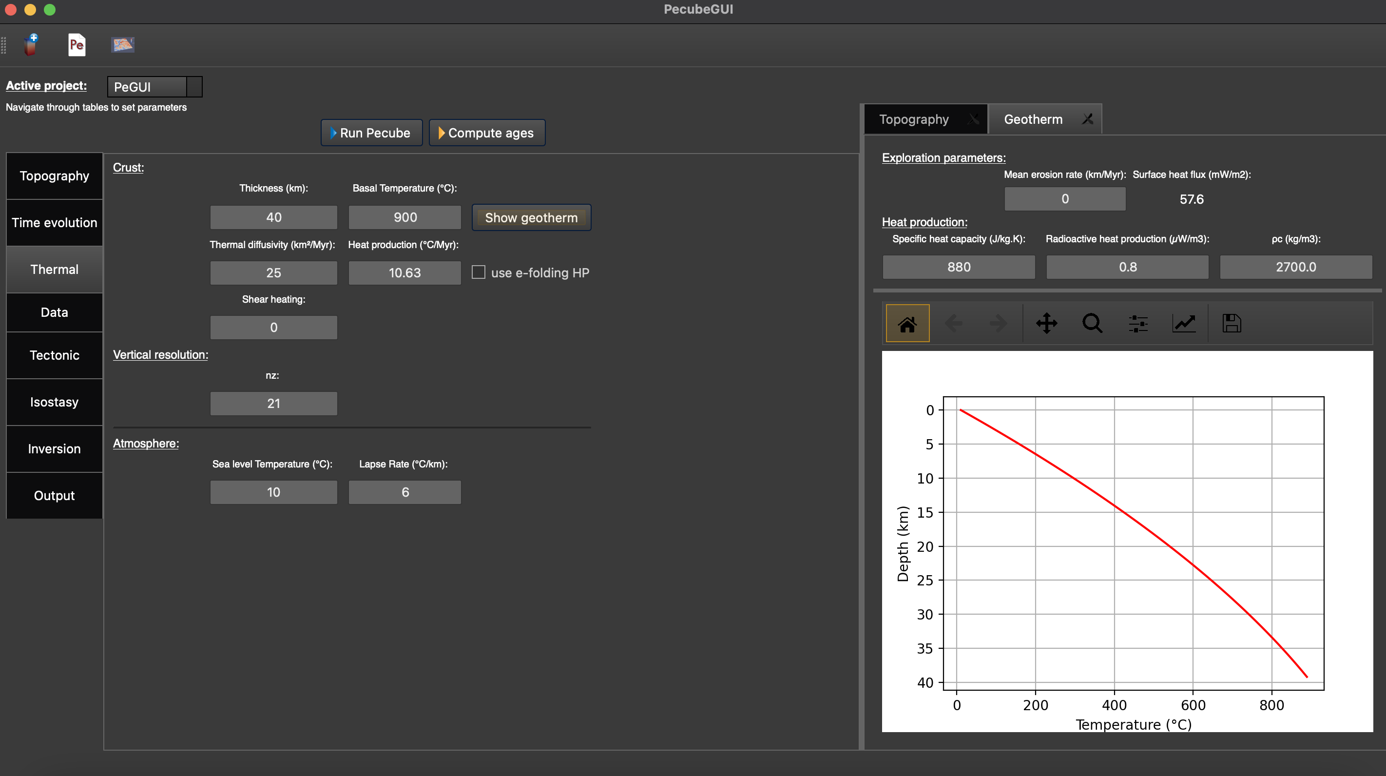
Figure 9. “Geotherm” tab where to provide parameters related to Thermal properties of the crust and the atmosphere.

Data tab

---

The first part (i.e., “Compute ages”) let you choose between three options:

• none: Pecube will not predict any thermochronological ages

• for all nodes: Pecube will predict thermochronological ages for all nodes at the surface of the Pecube model.

• sample specific: Pecube will predict thermochronological ages only at specific sample locations provided by the user.

Choosing ‘sample specific’ allows to provide the location of sample(s) from where to extract the thermal paths to compute ages at these specific locations. The user provides the name of the directory in “Data folder name” where the required file with the locations and observations will be stored. Then, the table below needs to be filled by providing the number of samples (Figure 10), and their respective coordinates (latitude and longitude), elevation, and the number of observation for each thermochronometers.

Warning

The ID of a sample must not include space !

Finally you can check for your sample location on the input topography by clicking on “Check sample locations”, as well as the predicted elevation of the samples on the input DEM (potentially degraded with ‘nskip’ parameter) by clicking on ‘Check sample elevations’.

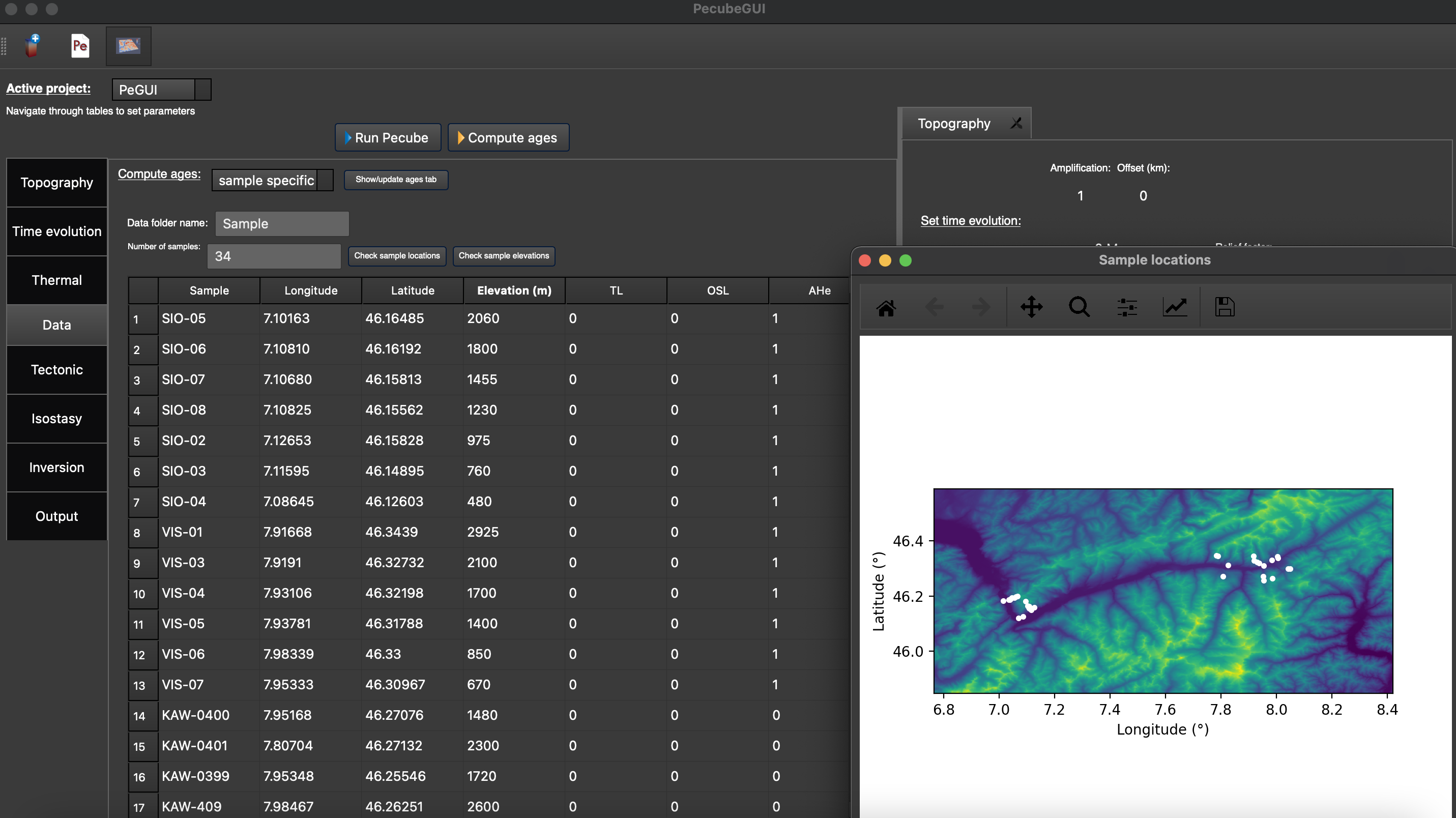
Figure 10. “Data” tab where to provide the sample location(s) and number of observations for each thermochronometers. The extra window shows the location of the samples, here in the Rhone valley area (data from Valla et al., 2012)

After providing the number of observations, you can click on ‘Show/update ages tab. A tab will open, where you can provide information for each thermochronometer (Figure 11).

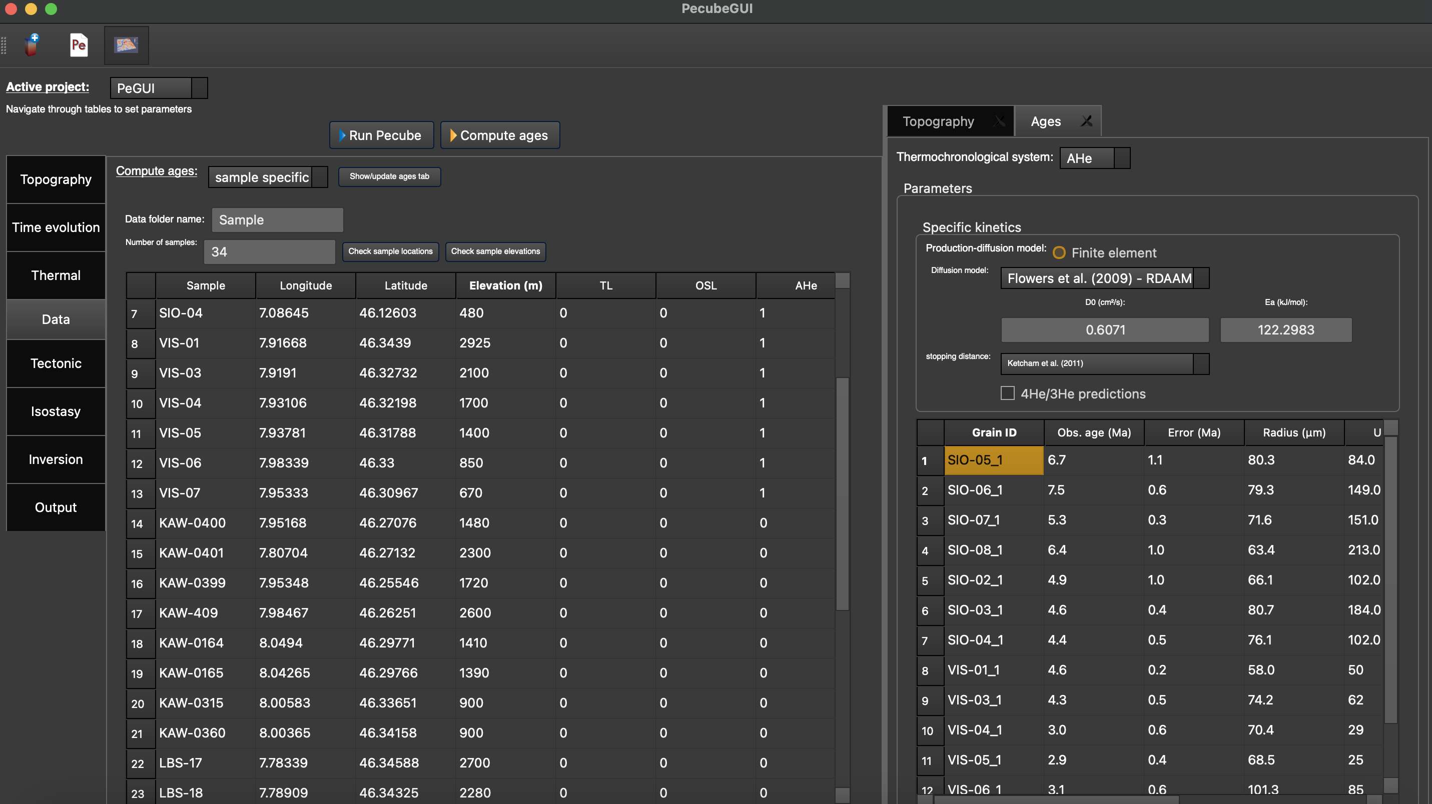
Figure 11. “Ages” tab where to define the thermochronometers to use. Here, the example is made with sample specific predictions for the apatite (U-Th)/He system.

Here you can provide observations (ages with uncertainties), and show extra parameters for the computation of grain-specific ages.

Apatite (U-Th)/He (AHe)

The “AHe” section show all the kinetic parameters related to the apatite (U-Th)/He thermochronometer:

• Diffusion model: the helium diffusion model to use. The options are the Farley et al. (2000), Shuster et al. (2006), and the radiation-damage models from Gautheron et al. (2009), Flowers et al. (2009, RDAAM) and Willett et al. (2017, ADAM).

• Ea: The activation energy (kJ.mol^-1). Ea is automatically updated according to the selected diffusion model, but it can be changed at the user’s discretion.

• D0: the diffusivity parameter value for infinite temperature (cm².s^-1). The value is updated according to the diffusion model selected.

• stopping distances: stopping distances for alpha particules from Farley et al. (1996) or Ketcham et al. (2011).

• 4He/3He predictions: enables prediction of ⁴He/³He profiles for each grain. When checked, a new window opens. Within this window, you can provide your heating schedule, with the number of steps, or let the default heating schedule. This will be used in the diffusion model to simulate a degassing experiment and compute ⁴He/³He ratios. The heat is in °C and the duration in hours.

• Table of observations: The table includes the observed ages and their uncertainties, the size (radius) of the grains, their uranium and thorium concentration (in ppm), and the fission track annealing kinetic parameters (only for Flowers et al. (2009) and Gautheron et al. (2009) diffusion models). In the current version, the grain is assumed spherical.

Apatite 4He/3He thermochronometry

Enabling ⁴He/³He prediction opens a window from which to provide observed spectra (Figure 12). The window starts with an information text explaining how to provide each spectrum. The steps are: 1. Select the grain from wich to provide an observed ⁴He/³He profile, 2. Set the number of heating steps, 3. Provide the heating schedule (optional), time is in hours and temperature in Celsius degree. 4. Provide the cumulative sum of fractional 3He (F3He) with the associated uncertainty (Error F). 5. Provide the 4He/3He ratio (i.e., Rs/Rb: Rstep/Rbulk) with its associated uncertainty (Error R). 6. Click on ‘add grain’ to add the ⁴He/³He profile for the selected grain. The grain’s ID is shown on the list in 7. To remove a ⁴He/³He profile for a grain, select the targeted grain on the list in 7 and click on “Remove grain” (8). Once, all 4He/3He profiles for targeted grain are provided click on the Ok button to save the profiles. The input file with ⁴He/³He data is then saved in your Pecube project folder “Project_name/data/data_folder_name/He43_data.csv”.

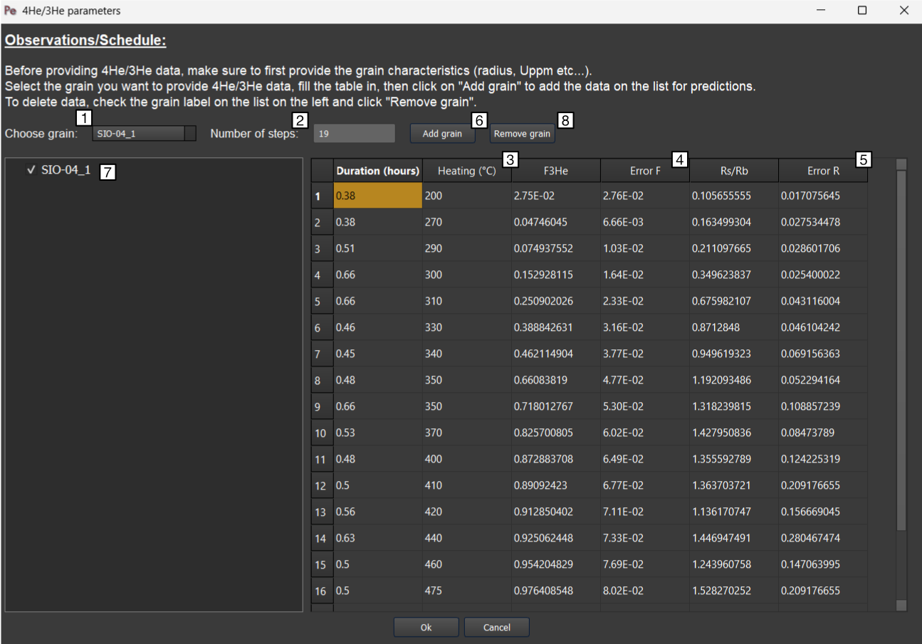
Figure 12. Providing observed 4He/3He profile within PecubeGUI. see main text for details.

Apatite fission track (AFT)

In the “AFT” section, the variable input parameters are:

• Annealing model: the model for annealing of fission tracks ([Ketcham-2007])

• Use FTL: option to use fission track length in the misfit calculation (for inversion mode)

• Kinetic parameter: the kinetic parameter to use to compute annealing and initial fission track length. The options are Dpar (µm), Cl (apfu), OH (apfu), Cl (wt %), rmr0

• Density reduction in standard: the ratio between spontaneous and induced track lengths in the standard used for calibration (Default: Durango).

• Table of observations: Within this table you can provide the observed (central) ages and their uncertainties, along with the kinetic value for each apatite group, and the mean fission track length (MFTL) with the standard deviation value associated. The two last observations are not mandatory.

In the current version of Pecube, the annealing model is restricted to the [Ketcham-2007] model. For the MFTL, only the c-axis projected value are predicted. As such, the user has to provide the observed c-axis projected MFTL in the table. The inital track length is calculated based on the kinetic parameter value according to [Carlson-1999].

Zircon (U-Th)/He (ZHe)

In the “ZHe” section, the input parameters comprise:

• Diffusion model: the helium diffusion model. Two models are included so far: [Reiners-et-al-2004] and [Guenthner-et-al-2013], The latter account for the radiation damages effect on helium diffusion.

• Ea: The activation energy (kJ.mol^-1). This is automatically updated according to the selected diffusion model, but it can be changed at the user’s discretion.

• D0: the diffusivity parameter value for infinite temperature (cm².s^-1). The value updates according to the selected diffusion model.

• stopping distances: stopping distances for alpha particules from Farley et al. (1996) or Ketcham et al. (2011).

• Table of observations: The table includes the observed ages and their uncertainties, the size (radius) of the grains, their uranium and thorium concentration (in ppm, only used in the Guenthner diffusion model). In the current version, the grain is assumed spherical.

Zircon fission track (ZFT)

The “ZFT” section is relatively simple and in the current version does not allow for many choices. The annealing model is based on a zero-damaged zircon from [Rahn-et-al-2004]. The input parameter only include:

• Table of observations: The table includes the observed ages and their uncertainties used to plot observed vs predicted ages.

Ar-Ar systems (BAr, KAr, MAr, HAr)

For the Ar-Ar themochronometric systems (BAr, MAr, KAr, HAr), the sections are similar and relatively simple:

• Ea: The activation energy (kJ.mol^-1). This is automatically updated according to the selected diffusion model, but it can be changed at the user’s discretion.

• D0: the diffusivity parameter value for infinite temperature (cm².s^-1). The value updates according to the selected diffusion model.

Default values for Ea and D0 are from [Grove_and_Harrison-1996] (BAr), [Hames-and-Bowring-1994] (MAr), [Harrison-1981] (HAr), and [Lovera-et-al-1991] (KAr).

Tectonic tab

---

This tab is related to the “Tectonic parameters” in the Pecube user guide. At the top of the tab three options are available:

• no uplift: compute the effect of topographic change only on thermal field

• bloc uplift: vertically uniform movement of the entire domain

• faulting: rock advection along fault(s)

According to the option chosen, you will have access to different part of the tab. For a bloc uplift, you can define the magnitude of the uplift rate at each corner of the model domain (i.e., bottom left, bottom right, top left, and top right). The uplift history is defined by the number of step (i.e., ‘nstep’) and the time window defined in the table below.

When faulting is chosen, the button’ ‘set faults’ is enabled. Clicking on it open a window where you can define your fault(s) geometry. You need to provide the number of faults (‘nfaults’), the number of points that will define the geometry of each fault (‘npoints’), and the coordinates of the two points that define the orientation of the faults (see Pecube’s documentation for more details). Then you can define each geometry by setting the position and depth of each points of the fault according to the coordinates of the fault plane.

Note

1. To define the type of fault, we keep on the convention described in the Pecube’s documentation. To define a thrust the velocity has to be negative, a positive velocity means a normal fault (i.e., ‘velo’ in the table).

2. The order you define the position of the geometry points of the fault(s) matters. The convention is that the rock advection is set on the bloc to the right-hand side of the fault (see Pecube’s documentation for more details)

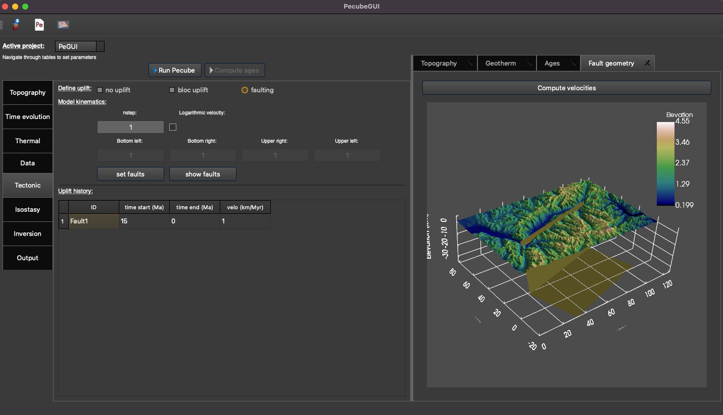
Figure 13. “Tectonic” tab where to provide parameters related to kinematic of rock uplift.

Inversion tab

---

In this tab, you will find parameters to:

• 1. control the inversion procedure

• 2. to use Pecube in Batch mode.

Pecube Batch mode has been introduced with the development of the PecubeGUI interface. Pecube Batch mode is useful to explore the effect of a single parameter on e.g. resulting age-elevation profiles. In this mode, Pecube run a couple of models by changing the value of a single parameter specified by the user as a range instead of a single value (i.e., using “min value: max value”) within a single Pecube project. To use Pecube in Batch mode, select “batch” in section “Choose inversion mode -> Inversion mode:”. Then, provide the number of intervals you wish to divide the parameter range values to. For instance, suppose a model designed as a bloc uplift with a single stage. One wish to investigate the effect of the exhumation rate in the resulting age-elevation profile. In this case, set the velocity (in Tectonic tab) to e.g., 0.2:2 km/Myr, then in “inversion tab” set the number of intervals to e.g., 4. Runing Pecube will launch 5 models with uplift rate values of [0.2, 0.65, 1.10, 1.55, 2.0] km/Myr. Once Pecube simulation is finished, go to the plotting area and load the Pecube project. In the list of available plots (see section “plot 2D data” below), you can choose “batch results” and choose to plot of interest. Plotting for instance the age-elevation profiles will show all the predicted age-elevation relationships related to each uplift rate value (i.e., [0.2, 0.65, 1.10, 1.55, 2.0]) on a single plot.

Alternatively, one can choose to run Pecube in inversion mode. Pecube is coupled with the Neighborhood algorithm [Sambridge-et-al-1999] that manages the inversion procedure. The inversion mode of Pecube is used to search for a range or a combination of parameter values that optimizes the fit to the data (i.e., or that minimizes the misfit). Controlling parameters for the NA algorithm are listed in the sub-section “Iteration performance” of PecubeGUI. These are:

• Number of cores: set the number of thread to use during the inversion (= number of forward models to run in parallel). This is used to run the command mpiexec -np n bin/PecubeMPI.sh NAME, where np is the number of cores/threads.

• Maximum number of iterations: the maximum number of iteration you want to perform. One iteration correspond to a set of pecube forward models (see after).

• Sample size for the first iteration: number of Pecube forward models to run in the 1st iteration.

• Sample size for all other iteration: number of Pecube forward models to run in all other iterations.

• Number of cells to resample: Number of Voronoi cells to resample at the start of each iteration. The NA algorithm will sample the nth Voronoi cells showing the lowest misfit. The ratio between the number of cells to resample and the sample size for all other iteration set the exploration efficiency of the parameter space by the algorithm. A ratio of 50-90% is usely recommanded, where the higher the ratio the more explorative is the algorithm (see [Braun-et-al-2012] for more details).

The last section of the tabs enables to set and control the misfit function used for inversion. The inversion procedure compares the predictions with the observed data through a misfit function (i.e., to minimize). The user can choose the misfit function to use:

• Chi-squared (default): \(\phi_1 = \sum_{j=1}^{N}((\frac{S^{obs}_j - S^{pred}_j}{ \sigma_j})^2)\).

where \(S^{obs}_j\) the observed data j and \(S^{pred}_j\) the predicted data j, \(\sigma_j\) the error on the observed data j, and N the total number of observed data.

• Reduced Chi-squared: \(\phi_2 = \sum_{j=1}^{N}(\frac{\phi_1}{N - N_d - 1})\).

where \(N_d\) is the number of inverted parameters.

• L2-norm: \(\phi_3 = \sqrt{\phi_1}\).

• L1-norm: \(\phi_4 = \sum_{j=1}^{N}((\frac{abs(S^{obs}_j - S^{pred}_j}{ \sigma_j}))\). In the current Pecube version, L1-norm is automatically set to calculate misfit in ⁴He/³He data, regardless the misfit function chosen to calculate misfit for all other thermochronometers.

In addition to the misfit function, you can manually control the weight each thermochronometer data will have in the misfit calculation. For this, click on Misfit weight Age: and a new window appears. Inside, each thermochronometric system is shown with a box where you can set the weight for the thermochronometer. Default values are 1, decreasing the value reduces the weight for the thermochronometer, increasing the value increases the weight.

---

Run a Pecube model

To run a Pecube model, simply click on “Run Pecube” above the tabs (Figure 13). A new window pops up. According to your preferences (cf. ‘2’, “Introduction” Figure 1) the latter will only show a progress bar of the Pecube run (‘Show console’ unchecked in Preferences) or additional information are provided if the console is enabled (“Show console” checked in Preferences).

When the console is allowed to be shown, the state of the runs is written within it. At the end of the Pecube run, this window displays ‘Pecube run is finished!’ and you can click on the ‘Ok’ button to close the window.

Note that you can also choose to not run Pecube but only the external routine to predict ages for sample-specific locations from an old Pecube project. This is useful when one wants to use e.g., another radiation damage model and do not want to run Pecube again. To do so, simply click on “Compute ages” (Figure 13, this option is diabled temporarily).

Note

When several projects are opened, the consoles are gathered in a single window to have a quick overview of all the running simulations.

Plotting results

In that section, I provide an overview of the chart part of PecubeGUI. There, you can plot results from your Pecube run.

Plot 1D data

---

To plot modelling results in PecubeGUI, first switch to the chart’s window by clicking on ‘show ouput’ (see Figure 1 in “Introduction”, n°5). You should see the window shown in Figure 14. On the left-hand side, you will find two tabs: Data and Properties. The first tab enables to load new data:

• Load project…: load a Pecube input file to plot data from that project.

• Add 3D model…: load a vtk file to visualize a 3D model.

• Remove data…: remove one or several plots. To do so, on the plot list on the left-hand side of the interface, select the plot you wish to remove and click ‘Remove data…’.

• Further data…: a list of data you can plot.

In the current version, and depending on your input parameters, Pecube can output several files. These files are:

• CompareAge.csv: This file contains the predicted and observed ages as well as sample ID and coordinates.

• TimeTemperature.csv: stores the thermal path of each sample location you provided. For this file to be created, you also need to check ‘save PTT paths’ in the ‘Output parameters’ tab.

• CoolingRates.csv: contains the time-temperature paths from all nodes in the model (work in for all node mode, see Data tab). This file is created if the option “Cooling rates” is checked (see “Output tab”). This allow the user to plot a 2D map of cooling rates defining a temperature or time interval.

• PecubeXXX.vtk: This file is located in the “VTK” directory of your project. If loaded for 2D data plot, a window will show up and ask you which data to plot from the file. You can extract, for instance, the 2D spatial distribution of the temperature at a specified depth, or extract the depth of an isotherm.

• AgeXXX.vtk: This file is located in the “VTK” directory of your project. If loaded for 2D data plot, you can choose to plot the 2D spatial distribution of the erosion rate or the predicted ages, at the surface of the Pecube model (only with the “for all nodes” option, see Data tab).

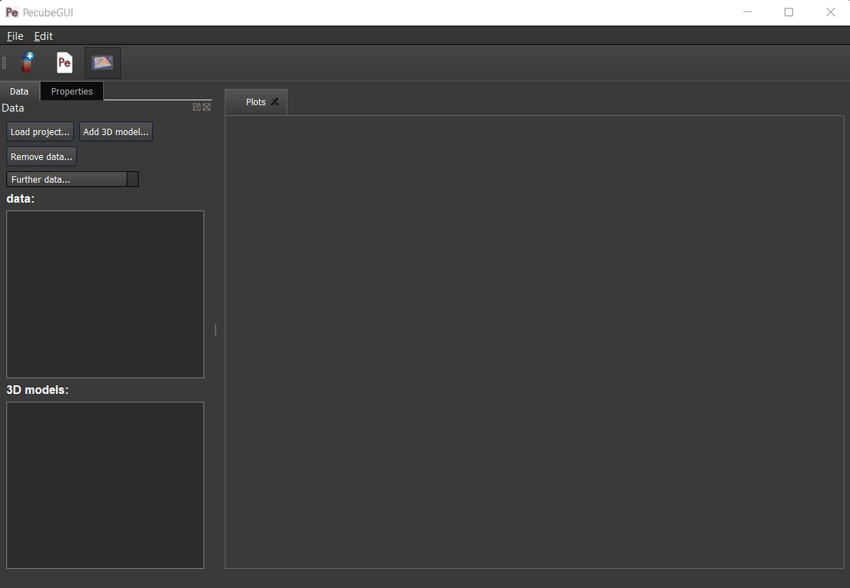
Figure 14. Chart’s window.

For each Pecube project, the data you can plot will be listed in “Further data…” (Figure 14). However, you first need to tell PecubeGUI which pecube project you want to work with. To do so, click on ‘Load project…’, then a window appears and ask you to choose an input file corresponding to the Pecube project you desire to plot from. After loading the input file, the list below will update and show you what kind of data you can plot. From there you could plot:

• Age-elevation: the ages plotted against elevation. If you computed ages for all surface nodes of the model, then you will be asked to choose at which time step(s) you want to plot data. If you computed ages at specific locations and for several thermochronometers, all of them will be plotted along with the observed data you provided. Then you will be free to show/hide data as you wish (see Figure 15).

• Date-eU: plot ages against effective uranium. Works only if you computed AHe or ZHe ages at specific locations.

• Age-comparison: plot observed vs predicted ages.

• Age transect: plot observed and predicted ages along a transect (Latitude, longitude, or projected).

• Tt paths: plot the thermal path of each sample. Works only if you computed ages at specific locations.

• 4He/3He data: plot either 4He/3He spectra or step ages profiles.

• 2D map of cooling rates: compute cooling rates for all surface node of the model (work only if mode *for all nodes”, see Data tab). You will be asked to define the temperature or time range on which you wish to calculate the cooling rates, as well as the interpolation method you want to use.

• 2D map of temperatures: plot the temperature/depth map at a certain depth/isotherm. To plot this map you will need to load one of the “PecubeXXX.vtk” file in the “VTK” directory of you pecube project.

• 2D map of Ages: plot the ages at the surface of the model. Works only if you computed ages for all surface nodes! To plot this map you will need to load one of the “AgesXXX.vtk” file in the “VTK” directory of you pecube project.

• Inversion results: plot the result of inversion. Four options are available: 1) Misfit evolution: plot the misfit value over each model run, 2) 2D parameter space: plot parameter X vs parameter Y in scatter plot where colors represent the misfit value. This option is enabled when running the sampling stage of the Neighborhood Algorithm (included in Pecube), 3) 2D parameter space + 1D PDF: similar to the previous point but with PDF shown for each parameter, and 4) PDF single parameter: show only the PDF for one parameter.

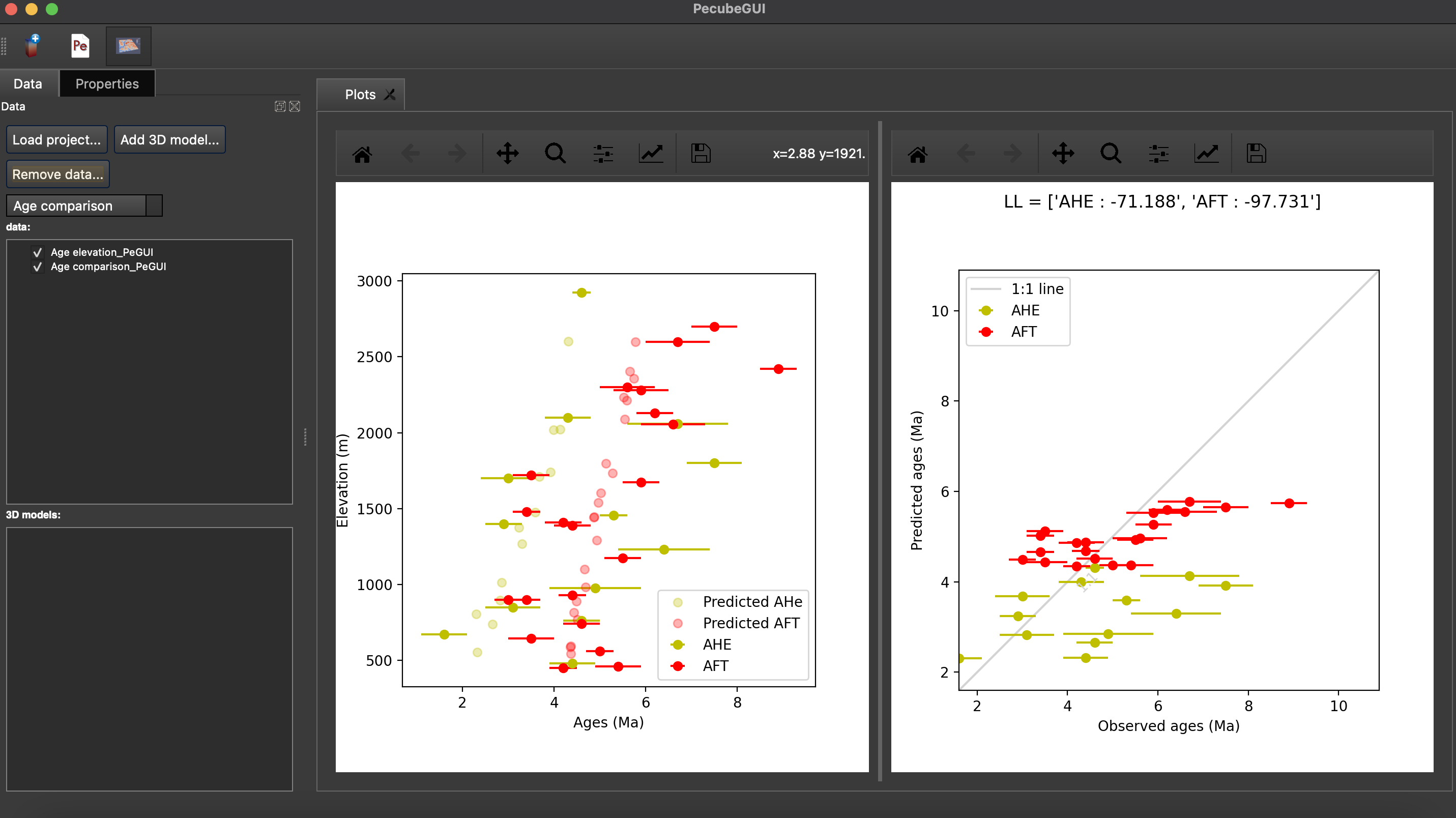
Figure 15. An example of PecubeGUI output. The first plot is the predicted and observed age vs elevation relationship for AHe and AFT ages from the Mont Blanc area, while the second is the “age comparison” plot where predictions are compared with observation. In this plot, the misfit value for each thermochronometer is shown.

Note

When plotting predictions from specific locations, and if observed data are provided, a misfit value between predicted and observed data is shown on the plot for each thermochronometer. The misfit value is the chi-squared, defined as: \(\phi = \sum_{j=1}^{N}((\frac{S^{obs}_j - S^{pred}_j}{ \sigma_j})^2)\). The log likelihood value is also shown and is the probability to have the observed data according to the model predictions. The log-likelyhood is defined following Braun et al. (2012): \(LL = -\sum_{j=1}^{N}(\frac{ln(2\pi)}{2}+ln(\sigma_j)+0.5(\frac{S^{obs}_j - S^{pred}_j}{ \sigma_j})^2\).

Where \(S^{obs}_j\) the observed data j and \(S^{pred}_j\) the predicted data j, \(\sigma_j\) the error on the observed data j, and N the total number of observed data. The higher the value of LL, the better is the match between observed and predicted data.

Visualize 3D models

---

PecubeGUI offers a 3D interactive interface where to visualize 3D models alongside with sample locations (if defined). The 3D interface is handling with pyvista [Sullivan-et-al-2019], which is an open-source package to read and manage vtk files.

To load a 3D model, click on “Add 3D model…” and select your vtk file from your Pecube project directory. A new tab will appear with a 3D environment and the 3D model (Figure 16).

If you chose to predict ages at specific locations, those locations will be automatically loaded with your 3D model. However, you can show/hide them by checking the box “show sample location(s)” on the properties tab (left side of the window, see Figure 16). On this tab, you have several options to set properties of the 3D model:

• Data range: set the range of data for the colorbar.

• Current data: list to choose the data to show (i.e., for the colormap).

• X, Y, Z scales: to scale the 3D model in the x, y, and z, directions.

• Reset camera position: reset the camera view to the initial position.

• Clear plot: remove the 3D model from the 3D interface.

• Export image…: save a screenshot of the 3D interface.

• Show box: to show the axes of the 3D model.

• Show sample location(s): to show/hide sample locations within the 3D interface.

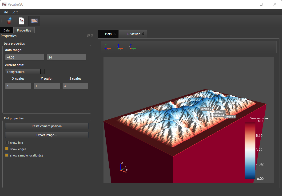
Figure 16. 3D viewer in PecubeGUI. An example is shown where the surface temperature is shown on the topography alongside with the sample locations that have been defined (see output tab).

References

[Braun-et-al-2012]

Braun, J., Van Der Beek, P., Valla, P., Robert, X., Herman, F., Glotzbach, C., … & Prigent, C. (2012). Quantifying rates of landscape evolution and tectonic processes by thermochronology and numerical modeling of crustal heat transport using PECUBE. Tectonophysics, 524, 1-28.

[Carlson-1999]

Carlson, W. D., Donelick, R. A., & Ketcham, R. A. (1999). Variability of apatite fission-track annealing kinetics: I. Experimental results. American mineralogist, 84(9), 1213-1223.

[Egholm_et-al-2011]

Egholm, D. L., Knudsen, M. F., Clark, C. D., & Lesemann, J. E. (2011). Modeling the flow of glaciers in steep terrains: The integrated second‐order shallow ice approximation (iSOSIA). Journal of Geophysical Research: Earth Surface, 116(F2).

[Gautheron-et-al-2010]

Gautheron, C., & Tassan-Got, L. (2010). A Monte Carlo approach to diffusion applied to noble gas/helium thermochronology. Chemical Geology, 273(3-4), 212-224.

[Grove-and-Harrison-1996]

Grove, M., & Harrison, T. M. (1996). 40Ar* diffusion in Fe-rich biotite. American Mineralogist, 81(7-8), 940-951.

[Guenthner-et-al-2013]

Guenthner, W. R., Reiners, P. W., Ketcham, R. A., Nasdala, L., & Giester, G. (2013). Helium diffusion in natural zircon: Radiation damage, anisotropy, and the interpretation of zircon (U-Th)/He thermochronology. American Journal of Science, 313(3), 145-198.

[Hames-and-Bowring-1994]

Hames, W. E., & Bowring, S. A. (1994). An empirical evaluation of the argon diffusion geometry in muscovite. Earth and Planetary Science Letters, 124(1-4), 161-169.

[Harrison-1981]

Mark Harrison, T. (1982). Diffusion of 40 Ar in hornblende. Contributions to Mineralogy and Petrology, 78, 324-331.

[Ketcham-2005]

Ketcham, R. A. (2005). Forward and inverse modeling of low-temperature thermochronometry data. Reviews in mineralogy and geochemistry, 58(1), 275-314.

[Ketcham-2007]

Ketcham, R. A., Carter, A., Donelick, R. A., Barbarand, J., & Hurford, A. J. (2007). Improved modeling of fission-track annealing in apatite. American Mineralogist, 92(5-6), 799-810.

[Lovera-et-al-1991]

Lovera, O. M., Richter, F. M., & Harrison, T. M. (1991). Diffusion domains determined by 39Ar released during step heating. Journal of Geophysical Research: Solid Earth, 96(B2), 2057-2069.

[Rahn-et-al-2004]

Rahn, M. K., Brandon, M. T., Batt, G. E., & Garver, J. I. (2004). A zero-damage model for fission-track annealing in zircon. American Mineralogist, 89(4), 473-484.

[Reiners-et-al-2004]

Reiners, P. W., Spell, T. L., Nicolescu, S., & Zanetti, K. A. (2004). Zircon (U-Th)/He thermochronometry: He diffusion and comparisons with 40Ar/39Ar dating. Geochimica et cosmochimica acta, 68(8), 1857-1887.

[Reiners-and-Brandon-2006]

Reiners, P. W., & Brandon, M. T. (2006). Using thermochronology to understand orogenic erosion. Annu. Rev. Earth Planet. Sci., 34, 419-466.

[Sambridge-et-al-1999]

Sambridge, M. (1999). Geophysical inversion with a neighbourhood algorithm—I. Searching a parameter space. Geophysical journal international, 138(2), 479-494.

[Sullivan-et-al-2019]

Sullivan et al., (2019). PyVista: 3D plotting and mesh analysis through a streamlined interface for the Visualization Toolkit (VTK). Journal of Open Source Software, 4(37), 1450, https://doi.org/10.21105/joss.01450

[Piper-2021]

Piper, M. (2021). CSDMS Topography data component (Version 0.3.1) [Computer software]. https://doi.org/10.5281/zenodo.4608653